How to plot a function in MatLab | Example with Source codes

How to plot a function in MatLab?

In MatLab, plotting a function is a simple task than any other computer language. The MATLAB function plot can be used to construct graphs of two-dimensional functions. There are a lot of functions variest of the plot is available in MatLab language (function plot, 2D plot, 3D plot, and others). All plot-related functions are pre-defined in the MatLab language. Simply put the variable in the function and it will automatically create the plotline of the points. So, you need to download the MatLab software or you can use the online MathWorks compile to run the code. Previously we discussed a function named 'polyfit in MatLab', you can read it with description and source code. We are going to discuss how to plot a function in MatLab step by step.

how to plot a function in MatLab?

Plot a function in MatLab

You can plot the function like f(x) = x³ + x² + 1 over the interval [-2, 2] with an iteration of 0.02 using the following codes of lines:

x = [-2: 0.02: 2];
y = x.^3 + x.^2 + 1;
plot(x,y)

The plot is shown below figure.

Figure for the equation x³ + x² + 1

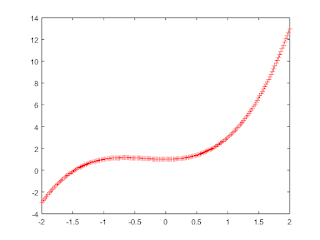
The plot(x,y,'r+:') statement will produce r=red with + for points and dotted line. For a variety of alternatives, use the help plot. Use 'g' for green, 'b' for blue, 'y' for yellow, and 'c' for cyan color. For coloring and styling the line of this above equation x³ + x² + 1,

change this,

plot(x,y)

with this,

plot(x,y, 'r+:')

And this will produce the below result,

After adding ' plot(x,y,'r+:')'

Other features can be added to a given graph to plot a function using functions of MatLab such as grid (horizontal and vertical line in the graph), x-label (naming the x-axis), y-label (naming the y-axis), title, etc. For example, if we add labels of the x-axis, y-axis, and title for the above equation x³ + x² + 1, then the code will be like this,

x = [-2: 0.02: 2];
y = x.^3 + x.^2 + 1;
plot(x,y, 'r+:')
xlabel('This is X axis');
ylabel('This is Y axis');
title('How to plot a function in MatLab?');

and output will be,

Adding x-label, y-label, and title in the graph in MatLab

Now, we want to add some horizontal and vertical lines to the plotted graph equation. This is very easy, we need to add the two words 'grid on'. That's all. And, by this, the plotting of a function in MatLab is completed. The full code is here,

x = [-2: 0.02: 2];
y = x.^3 + x.^2 + 1;
plot(x,y, 'r+:')
xlabel('This is X axis');
ylabel('This is Y axis');
title('How to plot a function in MatLab?');
grid on;

And the result is,

A full view to plot a function in MatLab with grid

3 steps to plot a function in MatLab (in short view)

1. Define x by giving the range of x values for which the function is to be plotted.

2. Create the function, y = f(x)

3. To draw a plot in MatLab, call the pre-defined plot function(x, y). plot(x,y).

How to plot sine and cosine curves in a graph in MatLab?

The plot function in MatLab takes multiple variables. So one can define multiple equations in the plot to draw a graph at a time. Now, we want to compare the sine and cosine curves in MatLab. Firstly,

declare the interval,

x=[0:0.01:3*pi];

then, assing the sine and cosine function in this interval,

y1=cos(x);
y2=sin(x);

Now, draw the curve,

plot(x,y1,x,y2)

full code for the sine and cosine comparison,

x=[0:0.01:3*pi];
y1=cos(x);
y2=sin(x);
plot(x,y1,x,y2)
legend('y1','y2')

Output figure is,

Plot sine and cosine function in MatLab

As there are two curves. So, we have added the legend to recognize the curve by coloring.

Legend in graph

How to plot a function in MatLab 3D view?

The function mesh creates three-dimensional or three-dimensional mesh surface plots. The function mesh(z) in MatLab generates a three-dimensional perspective plot of the matrix z's elements.

mesh(x,y,z)

3D plotting is easy to plot in MatLab same as the 2D plot. The mesh three-dimensional plot is very popular in terms of 3D-plot in MatLab. To use the mesh(z) function, we have to define the x, y, and z-axis points in mesh grids techniques. That is why, we will use the pre-defined meshgrid(x1,x2).

meshgrid(x1,x2);

The following example will generate the plot of the function z = e^{-(x^4 + y^4)}over the square [-5, 5] [-5, 5] with increment 0.1 shown in the below figure.

Code for 3D view in MatLab

[x y]=meshgrid(-5.0:0.1:5.0,-5.0:0.1:5.0);
z=exp(-x.^4-y.^4);
mesh(x,y,z)

Output figure,

3D plot of a function in MatLab

How to plot a function in MatLab | Example with Source codes