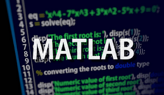
Calculate and plot with a bar of Histogram Normalization for an image in MatLab
% Read the input image using imread()
I=imread('matlab.PNG');

% If it is a color image
% Then, we need to turn it into a grayscale image
% Grayscale image will give a proper calculation
I=rgb2gray(I);
% Calculate the height and width of the input image
[height,width]=size(I);

% Compute the number of occurrences of each gray level
NumPixel = zeros(1,256);
for i = 1:height
    for j = 1:width
        % occurrences in the image
        NumPixel( I(i,j) + 1 ) = NumPixel( I(i,j) + 1 ) + 1;
    end
end


% Compute the probability of an occurrence of each gray level in the image
ProbPixel = zeros(1,256);
for i = 1:256
    % Calculating probability of each pixle
    ProbPixel(i) = NumPixel(i) / (height * width * 1.0);
end

bar(ProbPixel);
title('Normalized Histogram');
fprintf('Normalized Histogram calculated values are: \n');
fprintf('%f, ', ProbPixel);
Input Image
 |
| matlab.PNG |
Output Image
 |
| Normalized Histogram for the above image |
What is the Histogram Normalization process?
Normalizing a histogram is a technique that involves converting a discrete distribution of intensities into a discrete distribution of probability. To accomplish so, we must divide each histogram value by the number of pixels.
Application for Histogram Normalization
Photographs with low contrast due to glare, for example, can benefit from this technology. Normalization can also be referred to as contrast stretching or histogram stretching.
Histogram Normalization vs Histogram Equalization
They both yield comparable results but employ different methodologies. The normalization function is fairly basic; this technique looks for the highest intensity pixel and the lowest intensity pixel. Then calculates a factor that scales the lowest intensity to black and the highest intensity to white.
The Equalization function attempts to generate a histogram with an equal number of pixels in each intensity level.